
On the last article we have installed the Python Scikits library and run the samples provided. In this quick article we would like to find a candidate optimal trajectory that minimizes a weighted combination of speed and position values during a considered time interval $t_0=0$ s and $t_f=10$s. The performance measure $J(u)$ looks like this:
$$J(u) = \int_{t_0}^{t_f} {g(x(t),u(t),t)} dt$$
with $g(x(t),u(t),t)$ defined as:
$$g(x(t),u(t),t) = \dot{x}^2(t) + x^2(t)$$
This means that we would like to consider among all the possible trajectories connecting our initial and final points, only the ones that have small values of altitude and climbing speed. The Performance index becomes:
$$J(u) = \int_{t_0}^{t_f} {\dot{x}^2(t) + x^2(t)} dt$$
Since we would like to weight the velocity $\dot{x}(t)$ and the position $x(t)$ in the integral as we desire, we will add two coefficients $\alpha$ and $\beta$ as follows:
$$J(u) = \int_{t_0}^{t_f} {\alpha\dot{x}^2(t) + \beta x^2(t)} dt$$
By tuning the $\alpha$ and $\beta$ coefficients, we might select between all the possible trajectories only a bunch of them. We will see a couple of examples later.
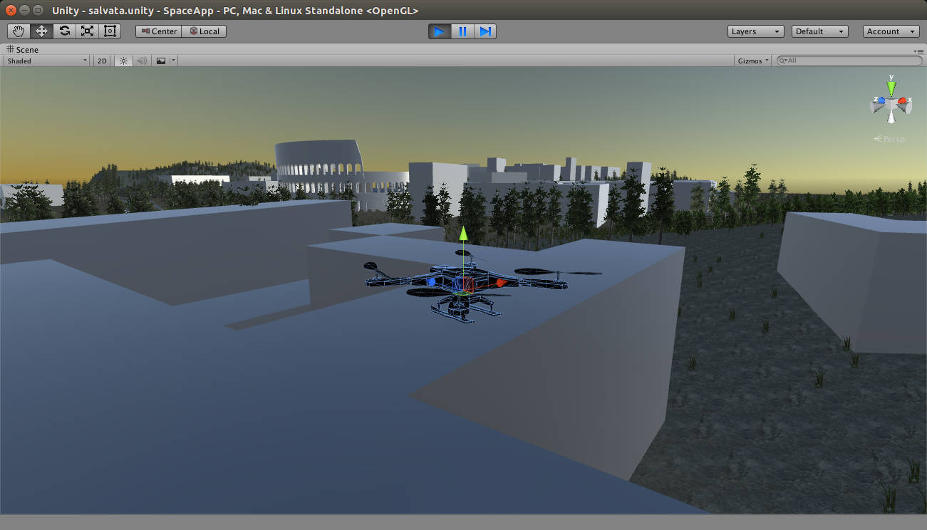
Let us consider the simplest problem with all the boundary conditions specified. We would like to reach 11 meters along the vertical axis starting from 0 in 10 seconds. So $t_0=0$ s, $t_f=10$ s, $x(0)=x_0=0$ m, $x(t_f)=x(10)=11$ m. Let’s consider an application of these kind of problem:
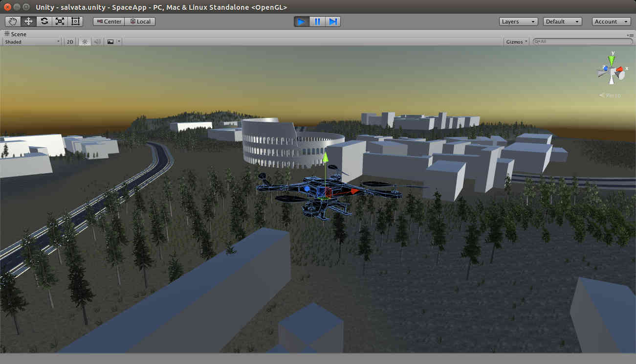
From X meters to X + 11 meters
For the trajectory $x(t)$ to be a minimizing function of the performance measure $J(u)$, it must be an extremal of $J(u)$. The variation of the performance index must be zero for all time instants in the considered interval.
$$ \delta J(u,\delta u) = \int_{t_0}^{t_f} {\frac{\partial g}{\partial x}-\frac{d}{dt}\left(\frac{\partial g}{\partial \dot{x}}\right)=0}$$
The resulting differential Euler-Lagrange equation will be:
$$ 2\beta x(t) – 2\alpha \ddot{x}(t) = 0$$
$$ \alpha \ddot{x}(t) = \beta x(t) $$
This is second order differential equation. Let’s redefine the problem in terms of first order differential equations. Let us call $x_1(t)$ the position and $\dot{x}$(t) the velocity of the body along the vertical $z$ axis.
$$\text{(1.1)} \quad \begin{cases}
\dot{x}_1(t) = x_2(t) & \\[2ex]
\dot{x}_2(t) = \left(\,\frac{\beta}{\alpha}\, \right) x_1(t),& &\text{$\forall$ $t$ $\in$ [$t_0$,$t_f$]}
\end{cases}$$
With $t_f$, $x(0)$ and $x(t_f)$ specified.
Python implementation
First, we need to import the bvp.solver and numpy. And set the Initial and final states. Remember that $x_1(t)$ is the altitude and $x_2(t)$ is the vertical speed.
Then we need to define the differential equation (1.1) to solve, the $\alpha$ and $\beta$ coefficients (let’s try with 1 and 1) and the boundary conditions:
Please note that the boundary condition function must return two numpy arrays that contains the difference between the actual boundary conditions and the required boundary conditions. The first array contains value of the left side $t_0$ and the second is related to the final conditions $t_f$. If you want to set an initial condition to the velocity on the left side, just change Ta[0] to Ta[1].
Next, create the ProblemDefinition object, by passing the relevant information and callbacks to its constructor:
And call the solve function to solve the boundary value problem. Pass the ProblemDefinition object and an initial guess for the solution. Here, we followed the suggestion for the initial guess provided by the official website. We used an array of constants for the guess, the average of the positions and the average of the velocity.
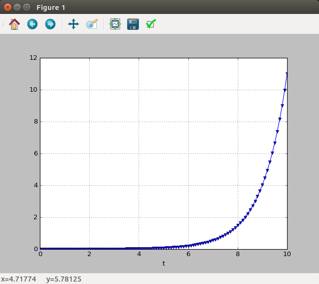
Finally, we can plot the result.
Ok this is the resulting trajectory. As you can see we start from $x_1(t_0)=0$ and we end up in $x_1(t_f)=11$ as desired but there is a problem, our velocity after 10 seconds is $x_2(t_f)=11 m/s$ which is not appropriate for our problem. The quadcopter’s position would go to infinity and we would end up by losing it.
If the vertical speed is not important
Modify the weights in our performance index with $\alpha=1$ and $\beta=100$ so that a small value of the vertical position $x_1(t)$ will cost 100 times more than $x_2(t)$
$$J(u) = \int_{t_0}^{t_f} {\dot{x}^2(t) + 100 x^2(t)} dt$$
The candidate optimal trajectory will penalize big values of the altitude and let speed assume important values. Since we need to reach 11 m at the end of the interval, we will have the vertical position close to zero for big amount of time and the an exponential increase in speed to reach the desired location. Here is what we get:
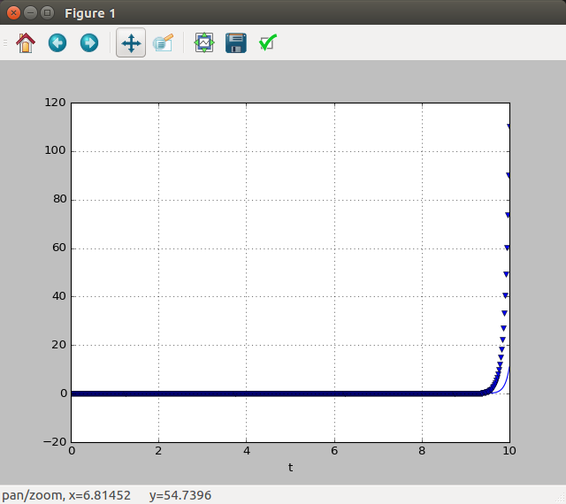
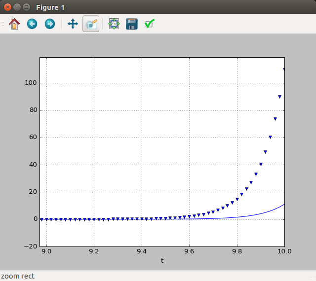
Let’s zoom a little bit near 10 seconds.
Small values of vertical speed
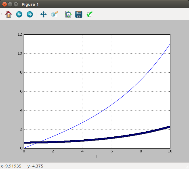
By weighting the $x_1(t)$ less than the $x_2(t)$ the trajectory is less aggressive.
$$J(u) = \int_{t_0}^{t_f} {\dot{x}^2(t) + 0.1 x^2(t)} dt$$
Modify the performance index as you wish
Feel free to add and modify the functional $J(u)$ to suit your needs. Below is another candidate optimal trajectory for a different performance index I have considered.
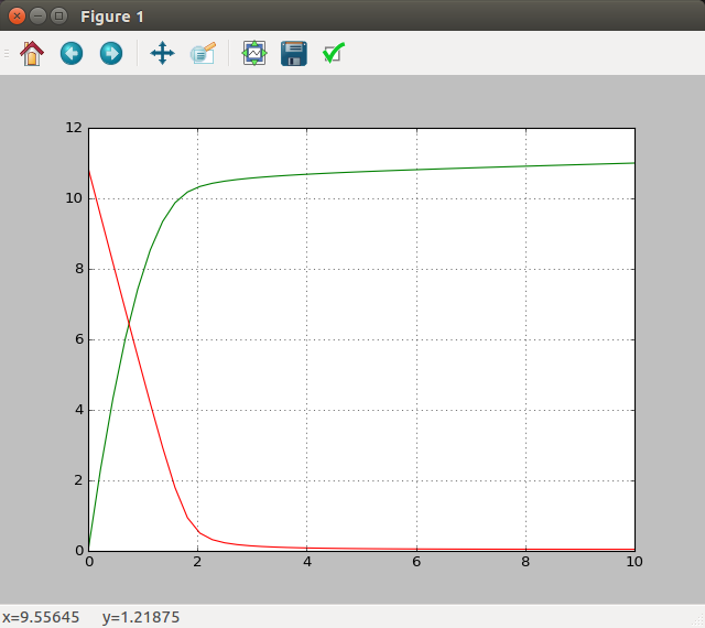
Hope this helps!